X-ray bursts and neutron star equation of state

Neutron stars (NSs) contain the most extreme forms of matter available in the Universe. They also serve as astrophysical laboratories to study physics under extreme conditions of strong gravity, ultrahigh densities, super-strong magnetic fields and high radiation densities. The densities in NS interiors can exceed the density of saturated nuclear matter (about 3 x 10¹⁴ g/cm³) by a large factor. One of the goals of modern physics is to understand the nature of the fundamental interactions. NSs serve as excellent natural laboratories to study strong interactions and to determine the most important properties of matter in atomic nuclei and NSs. The theory of quantum chromodynamics, which can, in principle, treat strong interactions, is computationally intractable for multi-nucleon systems at NS densities. Instead, physicists have developed empirical models of nucleonic interactions, which make conflicting predictions. Laboratory experiments and NS observations are vital to test these theories and drive the progress. NSs observations can be used to place constraints on strong interactions because the forces between the nuclear particles set the stiffness of NS matter. This is encoded in the equation of state (EoS), the relation between pressure and density. For a given NS mass M, the EoS sets its radius R via the stellar structure equations. By measuring the M-R relation, we can recover the EoS at supranuclear densities, which is of major importance to both fundamental physics and astrophysics. It is central to understanding NSs, supernovae, and compact object mergers including at least one NS. To distinguish among the models of strong interactions one needs to measure NS M and R to a precision of a few per cent for several NSs.

Our group has developed state-of-the-art neutron star atmosphere models and methods to measure NS parameters from the evolution of X-ray spectra observed during thermonuclear explosions at the NS surface known as X-ray bursts. For the first time, we have used the exact Compton scattering kernel to construct the most accurate atmosphere models for hot NSs (Suleimanov et al. 2012). We have proposed a novel “cooling tail” method to determine NS parameters. We have also discovered that the cooling tail properties strongly depend on the accretion rate and showed that only the low-accretion-rate, hard-state X-ray bursts can potentially be used for NS parameter determination (Kajava et al. 2014; Poutanen et al. 2014). Using the cooling tail method, we first found that the NS radius in a couple of known X-ray bursters is above 12.5 km (Suleimanov et al. 2011b; Poutanen et al. 2014), which supports stiff equation of state and is consistent with the existence of 2 solar mass pulsars. With the more advanced method of direct fitting atmosphere model to the data (Nättilä et al. 2017), we were able to the get the NS radius in 4U 1702-429 of R=12.4±0.4 km (see Fig. 1). The achived accuracy of the measurement of NS radius is much better than anything that was available before and even much better than is provided by the NICER mission, which is designed for that purpose.

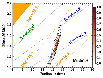
Figure 1: Constraints on the mass-radius of the neutron star in low-mass X-ray binary 4U 1702-429 from direct fits with the atmosphere model to the bursts cooling tail spectra. From Nättilä J. et al. (2017).

Our recent advance to the field includes the development of the NS atmosphere models for rapidly rotating stars accounting for the oblatness of the NS shape and variations of the gravity along the NS surface (Suleimanov et al. 2020, see Fig. 2). Constraints on the neutron star equation of state can also be obtained using pulse profiles of rotation-powered and accreting millisecond pulsars (AMPs) and from X-ray polarization to be observed from AMPs by the Imaging X-ray Polarimeter Explorer (IXPE) to be launched in the end of 2021.

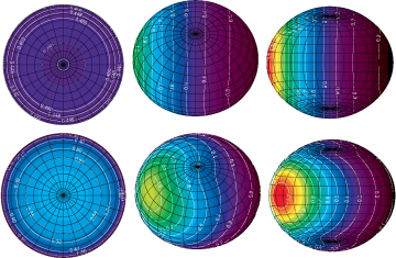
Figure 2: Images of a neutron star rotating at 700 Hz. Upper panels: blackbody case of local isotropic intensity. ower panels: electron-scattering dominated atmosphere. Panels from the left to the right correspond to the inclinations i= 0^o, 45^o, and 90^o. The lines of constant latitudes (every 10^o) and longitudes (every 15^o) are shown in black. From Suleimanov, Poutanen, Werner (2020).

• Suleimanov V.F., Poutanen J., Werner K.,
  Observational appearance of rapidly rotating neutron stars. X-ray bursts, cooling tail method, and radius determination,
  2020, A&A, 639,A33
• Sanchez-Fernandez C., Kajava J.J.E., Poutanen J., Kuulkers E., Suleimanov V.F.,
  Burst-induced coronal cooling in GS 1826−24. The clock wagging its tail,
  2020, A&A, 634, A58
• Suleimanov V.F., Poutanen J., Werner K.,
  Accretion heated atmospheres of X-ray bursting neutron stars,
  2018, A&A, 619, A114
• Suleimanov V.F., Kajava J.J.E., Molkov S.V., Nättilä J., Lutovinov A.A., Werner K., Poutanen J.,
  Basic parameters of the helium-accreting X-ray bursting neutron star in 4U 1820-30,
  2017, MNRAS, 472, 3905-3913
• Kajava J.J.E., Koljonen, K.I.I., Nättilä J., Suleimanov V.F., Poutanen J.,
  Variable spreading layer in 4U 1608-52 during thermonuclear X-ray bursts in the soft state,
  2017, MNRAS, 472, 78-89
• Nättilä J., Miller M.C., Steiner A.W., Kajava J.J.E., Suleimanov V.F., Poutanen J.,
  Neutron star mass and radius measurements from atmospheric model fits to X-ray burst cooling tail spectra,
  2017, A&A, 608, A31
• Kuuttila J., Kajava J.J.E., Nättilä J., Motta S.E., Sánchez-Fernández C., Kuulkers E., Cumming A., Poutanen J.
  Flux decay during thermonuclear X-ray bursts analysed with the dynamic power-law index method,
  2017, A&A, 604, A77
• Suleimanov V.F., Poutanen J., Nättilä J., Kajava J.J.E., Revnivtsev M.G., Wernee K.,
  The direct cooling tail method for X-ray burst analysis to constrain neutron star masses and radii,
  2017, MNRAS, 466, 906-913
• Kajava J.J.E., Sánchez-Fernández C., Kuulkers E., Poutanen J.
  X-ray burst-induced spectral variability in 4U 1728-34,
  2017, A&A, 599, A89
• Kajava J.J.E., Nättilä J., Poutanen J., Cumming A., Suleimanov V., Kuulkers E.,
  Detection of burning ashes from thermonuclear X-ray bursts,
  2017, MNRAS, 464, L6-L10
• Nättilä J., Steiner A.W., Kajava J.J.E., Suleimanov V.F., Poutanen J,
  Equation of state constraints for the cold dense matter inside neutron stars using the cooling tail method,
  2016, A&A, 591, A25
• Suleimanov V.F., Poutanen J., Klochkov D., Werner K.,
  Measuring the basic parameters of neutron stars using model atmospheres,
  2016, The European Physical Journal A, 52, 20
• Nättilä J., Suleimanov V.F., Kajava J.J.E., Poutanen J.,
  Models of neutron star atmospheres enriched with nuclear burning ashes,
  2015, Astronomy & Astrophysics, 581, A83
• in ‘t Zand J.J.M. (incl. Poutanen J.),
  The LOFT perspective on neutron star thermonuclear bursts,
  2015, white paper, arxiv:1501:02776
• Kajava J.J.E., Nättilä J., Latvala O.-M., Pursiainen M., Poutanen J., Suleimanov, V.F., Revnivtsev M.G., Kuulkers E., Galloway D.K.,
  The influence of accretion geometry on the spectral evolution during thermonuclear (type-I) X-ray bursts,
  2014, MNRAS, 445, 4218-4234
• Poutanen J., Nättilä J., Kajava J.J.E., Latvala O.-M., Galloway D.K., Kuulkers E., Suleimanov, V.F.,
  The effect of accretion on the measurement of neutron star mass and radius in the low-mass X-ray binary 4U 1608−52,
  2014, MNRAS, 442, 3777-3790
• Suleimanov V., Poutanen J., Werner K.,
  X-ray bursting neutron star atmosphere models using an exact relativistic kinetic equation for Compton scattering,
  2012, A&A, 545, A120
• Suleimanov V., Poutanen J., Revnivtsev M., Werner K.,
  Neutron star stiff equation of state derived from cooling phases of the X-ray burster 4U 1724−307,
  2011, ApJ, 742, 122
• Suleimanov V., Poutanen J., Werner K.,
  X-ray bursting neutron star atmosphere models: spectra and color corrections,
  2011, A&A, 527, A139